A Data-Driven Pizza Parlor

GOAL

RESULT

PROJECT DURATION

Adrian’s Pizzeria aims to enhance its pizza-making and optimize business operations through data-driven decision-making.

A comprehensive report with insights and recommendations for Adrian’s Pizzeria, facilitating well-informed decisions, cost savings, and process optimization.

The estimated duration of the project is 2 to 3 months, depending on the availability, completeness, and cleanliness of the data.

CASE – OPTIMIZING ADRIAN'S PIZZERIA OPERATIONS

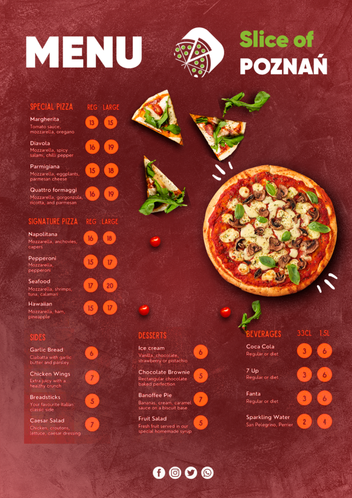
In the bustling world of pizzerias, there’s a hidden gem called “Slice of Poznań.” What sets Adrian’s apart isn’t just its mouthwatering pizzas but its dedication to data-driven decision-making.

The owner Adrian is on a mission to perfect his pizza-making game and optimize his business operations. Let’s dive into how Adrian’s Pizzeria uses data to make every slice count.

Orders: The Heart of the Business

At Slice of Poznań, every order tells a story, and Adrian wants to capture that narrative through data. Here’s what he needs:

Item name: To know what pizzas are popular.
Item price: To analyze pricing strategies.
Quantity: To track demand.
Customer name: For personalization.
Delivery address: To ensure popular locations
Row ID: A unique identifier for orders.
Order ID: A unique code for each customer’s order.
Item Name: The name of the ordered pizza.
Item Category: The pizza’s group, like “Vegetarian.”
Item Size: The pizza size (e.g., small, medium).
Item Price: The cost of the pizza.
Quantity: The number of pizzas ordered.
Customer First Name: Customer’s first name.
Customer Last Name: Customer’s last name.
Delivery Address: The address for pizza delivery.
Delivery City: The city for delivery.
Delivery Zip Code: The zip code for delivery location.

Stock Control: Keeping the Pantry Full

Adrian doesn’t want to run out of ingredients during the dinner rush. To prevent this, he needs:

Ingredients list for each pizza: To know what goes into each pizza.
Quantity of ingredients per pizza size: Plan inventory based on size.

Imagine making sure you have enough pepperoni and cheese for every pizza size; that level of accuracy is exactly what we’re aiming for.

Staff Control: Making Sure the Team Is Set

Adrian knows that his skilled chefs and delivery staff are key to his success. To manage his team effectively, he wants to:

Know which staff members are working and when: For efficient staffing.

By understanding labor costs, Adrian can make data-driven decisions on staffing and pricing.

Table Creation

Let’s begin by creating the necessary tables for MySQL usage.

CREATE TABLE `orders` (
`row_id` int NOT NULL ,
`order_id` varchar(10) NOT NULL ,
`created_at` datetime NOT NULL ,
`item_id` varchar(10) NOT NULL ,
`quantity` int NOT NULL ,
`cust_id` int NOT NULL ,
`delivery` boolean NOT NULL ,
`add_id` int NOT NULL ,
PRIMARY KEY (
`row_id`
)
);
CREATE TABLE `customers` (
`cust_id` int NOT NULL ,
`cust_firstname` varchar(50) NOT NULL ,
`cust_lastname` varchar(50) NOT NULL ,
PRIMARY KEY (
`cust_id`
)
);

CREATE TABLE `address` (
`add_id` int NOT NULL ,
`delivery_address1` varchar(200) NOT NULL ,
`delivery_city` varchar(50) NOT NULL ,
`delivery_zipcode` varchar(20) NOT NULL ,
PRIMARY KEY (
`add_id`
)
);

CREATE TABLE `item` (
`item_id` varchar(10) NOT NULL ,
`sku` varchar(20) NOT NULL ,
`item_name` varchar(100) NOT NULL ,
`item_cat` varchar(100) NOT NULL ,
`item_size` varchar(10) NOT NULL ,
`item_price` decimal(10,2) NOT NULL ,
PRIMARY KEY (
`item_id`
)
);

CREATE TABLE `ingredient` (
`ing_id` varchar(10) NOT NULL ,
`ing_name` varchar(200) NOT NULL ,
`ing_weight` int NOT NULL ,
`ing_meas` varchar(20) NOT NULL ,
`ing_price` decimal(5,2) NOT NULL ,
PRIMARY KEY (
`ing_id`
)
);

CREATE TABLE `recipe` (
`row_id` int NOT NULL ,
`recipe_id` varchar(20) NOT NULL ,
`ing_id` varchar(10) NOT NULL ,
`quantity` int NOT NULL ,
PRIMARY KEY (
`row_id`
)
);

CREATE TABLE `inventory` (
`inv_id` int NOT NULL ,
`item_id` varchar(10) NOT NULL ,
`quantity` int NOT NULL ,
PRIMARY KEY (
`inv_id`
)
);

CREATE TABLE `staff` (
`staff_id` varchar(20) NOT NULL ,
`first_name` varchar(50) NOT NULL ,
`last_name` varchar(50) NOT NULL ,
`position` varchar(100) NOT NULL ,
`hourly_rate` decimal(5,2) NOT NULL ,
PRIMARY KEY (
`staff_id`
)
);

CREATE TABLE `shift` (
`shift_id` varchar(20) NOT NULL ,
`day_of_week` varchar(10) NOT NULL ,
`start_time` time NOT NULL ,
`end_time` time NOT NULL ,
PRIMARY KEY (
`shift_id`
)
);

CREATE TABLE `rota` (
`row_id` int NOT NULL ,
`rota_id` varchar(20) NOT NULL ,
`date` datetime NOT NULL ,
`shift_id` varchar(20) NOT NULL ,
`staff_id` varchar(20) NOT NULL ,
PRIMARY KEY (
`row_id`
)
);

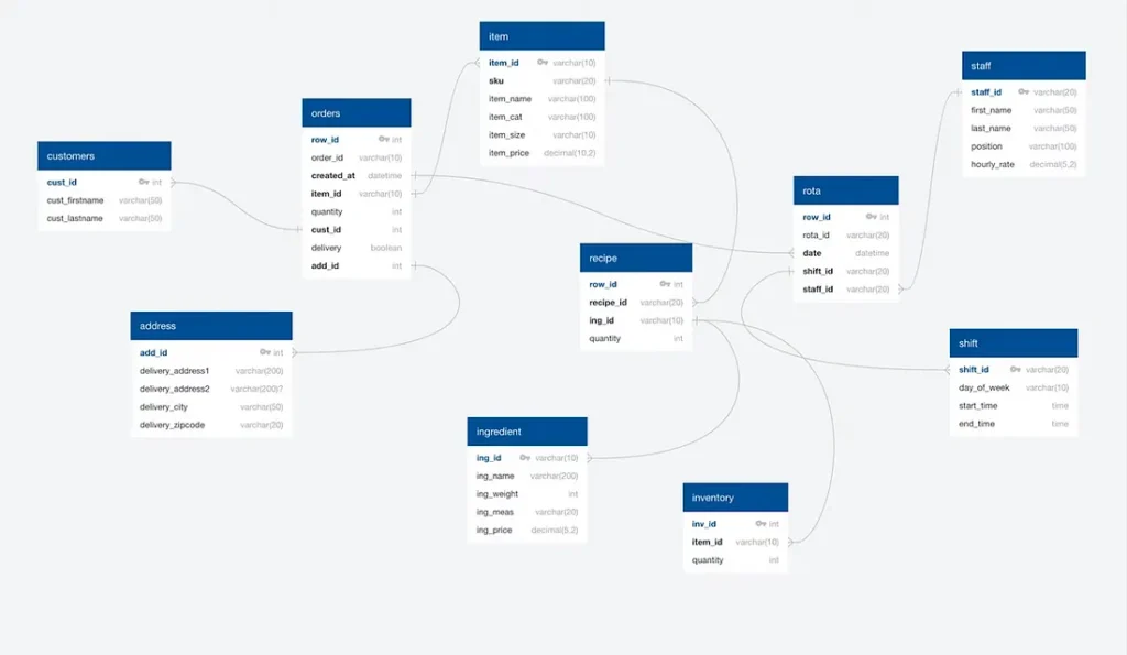
How tables look after they are created at QuickDatabaseDiagrams.com

Dashboards: Visualizing the Journey with Tableau

Now, let’s talk about the dashboards Adrian uses to make sense of all this data:

Dashboard 1: Order Activity

This dashboard provides a bird’s-eye view of Adrian’s Pizzeria:

Total orders: Tracking overall demand.
Total sales: Measuring revenue.
Total items: Understanding inventory usage.
Average order value: Analyzing spending habits.
Sales by category: Identifying popular pizza types.
Top selling items: Knowing customer favorites.
Orders by hour: Optimizing staffing.
Sales by hour: Identifying peak sales times.
Orders by address: Targeting delivery areas.

Adrian uses this dashboard to fine-tune his operations, from staffing to inventory management.

The SQL code I used to create the first dashboard, which we’ll call “Dashboard 1 — Orders.” This query retrieves data from various tables and joins them to provide insights into order activity. Here’s an explanation of the code:

SELECT
o.order_id,
i.item_price,
o.quantity,
i.item_cat,
i.item_name,
o.created_at,
a.delivery_address1,
a.delivery_city,
a.delivery_zipcode,
o.delivery
FROM
orders o
LEFT JOIN item i ON o.item_id = i.item_id
LEFT JOIN address a ON o.add_id = o.add_id

SELECT: Specifies the columns you want to include in the result set.
o.order_id: Retrieves the unique order ID.
i.item_price: Fetches the item price (pizza price).
o.quantity: Gets the quantity of items (number of pizzas) in the order.
i.item_cat: Retrieves the item category (e.g., “Vegetarian”).
i.item_name: Fetches the item name (pizza name).
o.created_at: Retrieves the order creation timestamp.
a.delivery_address1: Fetches the delivery address.
a.delivery_city: Retrieves the delivery city.
a.delivery_zipcode: Retrieves the delivery zip code.
o.delivery: Retrieves delivery-related data (possibly a status or method).

This query combines data from the “orders,” “item,” and “address” tables using LEFT JOINs based on the appropriate keys (e.g., order_id, item_id, add_id). It collects essential information about each order, including details about the pizzas, delivery, and customer addresses.

Dashboard 2: Inventory Management

This dashboard provides detailed information on the ingredients used and their respective costs.Total quantity by ingredient: Monitoring ingredient usage.

Total cost of ingredients: Tracking expenses.
Calculated cost of each pizza: Ingredient costs + labor costs.

By utilizing this data, Adrian can secure a constant supply of vital ingredients and make informed decisions about pizza pricing to maximize profits.

SQL Code for Inventory Analysis:

SELECT
    s1.item_name,
    s1.ing_id,
    s1.ing_name,
    s1.ing_weight,
    s1.ing_price,
    s1.order_quantity,
    s1.recipe_quantity,
    s1.order_quantity * s1.recipe_quantity AS ordered_weight,
    s1.ing_price / s1.ing_weight AS unit_cost,
    (s1.order_quantity * s1.recipe_quantity) * (s1.ing_price / s1.ing_weight) AS ingredient_cost
FROM
    (
        SELECT
            o.item_id,
            i.sku,
            i.item_name,
            r.ing_id,
            r.quantity AS recipe_quantity,
            SUM(o.quantity) AS order_quantity,
            ing.ing_weight,
            ing.ing_price,
            ing.ing_name
        FROM
            orders o
        LEFT JOIN
            item i ON o.item_id = i.item_id
        LEFT JOIN
            recipe r ON i.sku = r.recipe_id
        LEFT JOIN
            ingredient ing ON ing.ing_id = r.ing_id 
        GROUP BY
            o.item_id,
            i.sku,
            i.item_name,
            r.ing_id,
            r.quantity,
            ing.ing_name,
            ing.ing_weight,
            ing.ing_price
    ) s1;

Creating the Inventory View:

We begin by creating a view called “stock1” to work with the data more effectively:

CREATE VIEW stock1 AS
SELECT
    s1.item_name,
    s1.ing_id,
    s1.ing_name,
    s1.ing_weight,
    s1.ing_price,
    s1.order_quantity,
    s1.recipe_quantity,
    s1.order_quantity * s1.recipe_quantity AS ordered_weight,
    s1.ing_price / s1.ing_weight AS unit_cost,
    (s1.order_quantity * s1.recipe_quantity) * (s1.ing_price / s1.ing_weight) AS ingredient_cost
FROM
    (
        SELECT
            o.item_id,
            i.sku,
            i.item_name,
            r.ing_id,
            r.quantity AS recipe_quantity,
            SUM(o.quantity) AS order_quantity,
            ing.ing_weight,
            ing.ing_price,
            ing.ing_name
        FROM
            orders o
        LEFT JOIN
            item i ON o.item_id = i.item_id
        LEFT JOIN
            recipe r ON i.sku = r.recipe_id
        LEFT JOIN
            ingredient ing ON ing.ing_id = r.ing_id 
        GROUP BY
            o.item_id,
            i.sku,
            i.item_name,
            r.ing_id,
            r.quantity,
            ing.ing_name,
            ing.ing_weight,
            ing.ing_price
    ) s1;

Analyzing Remaining Ingredients:

Lastly, we calculate the total weight of inventory for each ingredient and determine how much is left in stock:

SELECT
    s2.ing_name,
    s2.ordered_weight,
    ing.ing_weight * inv.quantity as total_inv_weight,
    (ing.ing_weight * inv.quantity) - s2.ordered_weight as remaining_weight
FROM (SELECT 
    ing_id,
    ing_name,
    SUM(ordered_weight) as ordered_weight
    FROM 
    stock1
    GROUP BY ing_name, ing_id) s2
LEFT JOIN inventory inv ON inv.item_id = s2.ing_id
LEFT JOIN ingredient ing ON ing.ing_id = s2.ing_id;

This analysis allows Adrian’s Pizzeria to make informed decisions about restocking, ingredient costs, pricing, and profitability of each pizza.

Dashboard 3 — Staff Management: Tracking the Workforce

In this segment of Adrian’s Pizzeria’s data journey, we concentrate on managing the staff workforce, utilizing data from three critical tables: rota, staff, and shift.

SQL Code for Staff Analysis:

Step 1: Joining Rota and Staff Tables

We start by joining the “rota” and “staff” tables to create a comprehensive view of staff scheduling:

SELECT
    r.date,
    s.first_name,
    s.last_name,
    s.hourly_rate
FROM
    rota r
LEFT JOIN
    staff s ON r.staff_id = s.staff_id;

Step 2: Including Shift Information

Next, we add shift data to the mix, creating a more detailed picture of staff schedules:

SELECT
    r.date,
    s.first_name,
    s.last_name,
    s.hourly_rate,
    sh.start_time,
    sh.end_time
FROM
    rota r
LEFT JOIN
    staff s ON r.staff_id = s.staff_id
LEFT JOIN
    shift sh ON r.shift_id = sh.shift_id;

Step 3: Calculating Staff Costs

Lastly, we calculate the cost of staffing by determining the hours worked and multiplying them by the hourly rate using the TIMEDIFF() function:

SELECT
    r.date,
    s.first_name,
    s.last_name,
    s.hourly_rate,
    sh.start_time,
    sh.end_time,
    (
        (HOUR(TIMEDIFF(sh.end_time, sh.start_time)) * 60) + MINUTE(TIMEDIFF(sh.end_time, sh.start_time))
    ) / 60 AS hours_in_shift,
    (
        (
            HOUR(TIMEDIFF(sh.end_time, sh.start_time)) * 60
        ) + MINUTE(TIMEDIFF(sh.end_time, sh.start_time))
    ) / 60 * s.hourly_rate AS staff_cost
FROM
    rota r
LEFT JOIN
    staff s ON r.staff_id = s.staff_id
LEFT JOIN
    shift sh ON r.shift_id = sh.shift_id;

This data analysis helps Adrian’s Pizzeria efficiently manage its staff schedules and calculate the associated costs, ensuring a well-organized and cost-effective workforce.

You can access my imaginary datasets on my Github and Kaggle accounts for your use and modification.